Stochastic Differential Equations, Deep Learning, and High-Dimensional PDEs
Chris Rackauckas
January 18th, 2020
Now we will suss out the relationship between SDEs and PDEs and how this is used in scientific machine learning to solve previously unsolvable problems with a neural network as the intermediate.
What is an SDE?
The easiest way to understand an SDE is by looking at it computationally. For the SDE defined as:
\[ dX_t = f(X_t,t)dt + g(X_t,t)dW_t \]
the "Euler method for SDEs", also known as Euler-Maruyama, is given by:
\[ X_{n+1} = X_n + f(X_n,t_n)h + sqrt(h)g(X_n,t_n)\zeta \]
where $\zeta ~ N(0,1)$ is a standard normal random variable (randn()). Thus a stochastic differential equation is an ordinary differential equation with a small stochastic perturbation at every point in time (continuously!).
There are many definitions of Brownian motion. One of the easiest to picture is that it's the random walk where at every infinitesimal $dt$ you move by $N(0,dt)$ (this is formally true in non-standard analysis, see Radically Elementary Probability Theory for details). Another way to think of it is as a limit of standard random walks. Let's say you have a random walk were every time step of $h$ you move $\Delta x$ to the right or left. If you let $h/\Delta x = 1$ and send $h \rightarrow 0$, then the limiting process is a Brownian motion. All of the stuff about normal distributions just comes from the central limit theorem and the fact that you're doing infinitely many movements per second!
Wiener Process Calculus Summarized
Brownian motion is non-differentiable, and this is fairly straightforward to prove. Take any finite $h>0$. In that interval, the probability that the Brownian motion has a given value is $N(0,h)$. Thus it has a positive probability of being positive and a positive probability of being negative. Thus take the sequence $h/2$, $h/4$, etc. to have infinitely many subintervals. With probability 1 at least one of those values will be positive and at least one will be negative, and so for every $h$ there is a positive or negative value, which means Brownian motion is always neither increasing or decreasing. This means that, if the classical derivative existed, it must be zero, which means it's a constant function, but it's not, so by contradiction Brownian motion cannot have a classical derivative!
However, with a bunch of analysis one can derive an appropriate calculus on SDEs. Take the SDE
\[ dx=f(x,t)dt+\sum_{i=1}^{n}g_{i}(x,t)dW_{i} \]
where $W_{i}(t)$ is a standard Brownian motion. Ito's Rules (the stochastic chain rule) could be interpreted as:
\[ dt\times dt=0 \]
\[ dW_{i}\times dt=0 \]
\[ dW_{i}\times dW_{i} = dt \]
\[ dW_{i}\times dW_{j} = 0\,\,\,\,j\neq i \]
and thus if $y=\psi(x,t)$, Ito's rules can be written as:
\[ dy=\frac{\partial\psi}{\partial t}dt+\frac{\partial\psi}{\partial x}dx+\frac{1}{2}\frac{\partial^{2}\psi}{\partial x^{2}}\left(dx\right)^{2} \]
where, if we plug in $dx,$ we get
\[ dy=d\psi(x,t)=\left(\frac{\partial\psi}{\partial t}+f(x,t)\frac{\partial\psi}{\partial x}+\frac{1}{2}\sum_{i=1}^{n}g_{i}^{2}(x,t)\frac{\partial^{2}\psi}{\partial x^{2}}\right)dt+\frac{\partial\psi}{\partial x}\sum_{i=1}^{n}g_{i}(x,t)dW_{i} \]
Notice that this is the same as the normal chain rule formula, but now there is a second order correction to the main variable. The solution is given by the integral form:
\[ x(t)=x(0)+\int_{0}^{t}f(x(s))ds+\int_{0}^{t}\sum_{i=1}^{m}g_{i}(x(s))dW_{i}. \]
Note that we can also generalize Ito's lemma to the multidimensional
\[ \mathbf{X}\in\mathbb{R}^{n} \]
case:
\[ d\psi(\mathbf{X})=\left<\frac{\partial\psi}{\partial\mathbf{X}},f(\mathbf{X})\right>dt+\sum_{i=1}^{m}\left<\frac{\partial\psi}{\partial\mathbf{X}},g_{i}(\mathbf{X})\right>dW_{i}+\frac{1}{2}\sum_{i=1}^{m}g_{i}(\mathbf{X})^{T}\nabla^{2}\psi(\mathbf{X})g_{i}(\mathbf{X})dt \]
There are many other rules as well:
Product Rule: $d(X_{t}Y_{t})=X_{t}dY+Y_{t}dX+dXdY$.
Integration By Parts: $\int_{0}^{t}X_{t}dY_{t}=X_{t}Y_{t}-X_{0}Y_{0}-\int_{0}^{t}Y_{t}dX_{t}-\int_{0}^{t}dX_{t}dY_{t}$.
Invariance: $\mathbb{E}\left[\left(W(t)-W(s)\right)^{2}\right]=t-s$ for $t>s$.
Expectation: $\mathbb{E}[W(t_{1})W(t_{2})]=\min(t_{1},t_{2})$.
Independent Increments: $\mathbb{E}\left[\left(W_{t_{i}}-W_{s_{1}}\right)\left(W_{t_{2}}-W_{s_{2}}\right)\right]=0$ if $\left[t_{1},s_{1}\right]$ does not overlap $\left[t_{2},s_{2}\right]$.
Expectation of the Integral: $\mathbb{E}\left[\int_{0}^{t}h(t)dW_{t}\right]=\mathbb{E}\left[h(t)dW_{t}\right]=0$.
Ito Isometry: $\mathbb{E}\left[\left(\int_{0}^{T}X_{t}dW_{t}\right)\right]=\mathbb{E}\left[\int_{0}^{T}X_{t}^{2}dt\right]$
Example Problem: Geometric Brownian Motion
Look at the example stochastic process:
\[ dx=\alpha xdt+\sigma xdW. \]
To solve this, we start with our intuition from Newton's Calculus that this may be an exponential growth process. Thus we check Ito's equation on the logarithm $\psi(x,t)=\ln(x)$ for this process is,
\[ \begin{eqnarray*} d\left(\ln x\right) & = & \left(0+\left(\alpha x\right)\left(\frac{1}{x}\right)-\frac{1}{2}\left(\sigma^{2}x^{2}\right)\left(\frac{1}{x^{2}}\right)\right)dt+\left(\frac{1}{x}\right)\left(\sigma x\right)dW\\ d\left(\ln x\right) & = & \left(\alpha-\frac{1}{2}\sigma^{2}\right)dt+\sigma dW. \end{eqnarray*} \]
Thus by taking the integral of both sides we get
\[ \ln(x)=\left(\alpha-\frac{1}{2}\sigma^{2}\right)t+\sigma W(t) \]
and then exponentiating both sides:
\[ x(t)=e^{\left(\alpha-\frac{1}{2}\sigma^{2}\right)t+\sigma W(t)}. \]
Notice that since the Wiener process $W(t)\sim N(0,t)$, the log of $x$ is distributed normally as $N(\left(\alpha-\frac{1}{2}\sigma^{2}\right)t,\sigma^{2}t)$. Thus $x(t)$ is distributed as what is known as the log-normal distribution.
Example Numerical Solution of Geometric Brownian Motion
using StochasticDiffEq, Plots
p = (μ=1.0,σ=1.0)
f(u,p,t) = p.μ*u
g(u,p,t) = p.σ*u
prob = SDEProblem(f,g,1.0,(0.0,1.0),p)
sol = solve(prob,SRIW1())
plot(sol)

and automatic parallelism of the solution:
using DiffEqBase.EnsembleAnalysis
enprob = EnsembleProblem(prob)
# Note: Automatically parallel! Try on the GPU with EnsembleGPUArray() from DiffEqGPU.jl!
ensol = solve(enprob,SRIW1(),trajectories=10000)
summ = EnsembleSummary(ensol)
plot(summ)

SDEs as Regularized ODEs and Neural Stochastic Differential Equations
Since SDEs have inherent randomness to them, trivially it follows that they tend to not overfit data since, if they try to fit weird aspects of the data too closely, the randomness will wash out any attempt. This was noticed awhile back as a method for improving parameter estimation of determinsitic systems, and now is being revived as a tool for neural ODEs. The result is the neural SDE, which is a form of neural ODE where each trajectory is random.
To start, let's first build a training dataset from some true SDE. Here let's use the SDE:
\[ du_t = Au^3dt + 0.2dW_t \]
with diagonal noise (i.e., it's a system of equations, but each equation has its own noise term).
using Flux, DiffEqFlux, StochasticDiffEq, Plots, DiffEqBase.EnsembleAnalysis, Statistics

u0 = Float32[2.; 0.]
datasize = 30
tspan = (0.0f0,1.0f0)

function trueSDEfunc(du,u,p,t)
    true_A = [-0.1 2.0; -2.0 -0.1]
    du .= ((u.^3)'true_A)'
end
t = range(tspan[1],tspan[2],length=datasize)
mp = Float32[0.2,0.2]
function true_noise_func(du,u,p,t)
    du .= mp.*u
end
prob = SDEProblem(trueSDEfunc,true_noise_func,u0,tspan)
SDEProblem with uType Array{Float32,1} and tType Float32. In-place: true
timespan: (0.0f0, 1.0f0)
u0: Float32[2.0, 0.0]
Our dataset will be the means and variances from 100,000 runs:
# Take a typical sample from the mean
ensemble_prob = EnsembleProblem(prob)
ensemble_sol = solve(ensemble_prob,SOSRI(),trajectories = 10000)
ensemble_sum = EnsembleSummary(ensemble_sol)
sde_data,sde_data_vars = Array.(timeseries_point_meanvar(ensemble_sol,t))
(Float32[2.0 1.9701736 … 0.4452727 0.5757192; 0.0 0.54078853 … -1.101216 -0
.99688226], Float32[0.0 0.005057836 … 0.9892878 0.9156186; 0.0 0.0012974117
 … 0.48924 0.6094276])
Now let's build the neural SDE. In its general form,
\[ dX_t = f(X_t,t)dt + g(X_t,t)dW_t \]
we will specify both $f$ and $g$ as neural networks, but define the noise term $g$ to be diagonal noise, matching the data generation process.
drift_dudt = Chain(x -> x.^3,
             Dense(2,50,tanh),
             Dense(50,2))
diffusion_dudt = Chain(Dense(2,2))
n_sde = NeuralDSDE(drift_dudt,diffusion_dudt,tspan,SOSRI(),saveat=t,reltol=1e-1,abstol=1e-1)
ps = Flux.params(n_sde)
Params([Float32[0.2926085, 0.13294399, 0.25695634, -0.17434904, 0.17872418,
 -0.25109446, 0.21020114, 0.3169294, 0.17797352, 0.26585048  …  0.13026121,
 0.2738877, 0.0, 0.0, -0.4945196, 1.097075, -0.6068662, 0.5683143, 0.0, 0.0
], Float32[0.2926085 0.06574465; 0.13294399 0.007055972; … ; 0.1643526 0.00
9358183; -0.28269428 0.15322818], Float32[0.0, 0.0, 0.0, 0.0, 0.0, 0.0, 0.0
, 0.0, 0.0, 0.0  …  0.0, 0.0, 0.0, 0.0, 0.0, 0.0, 0.0, 0.0, 0.0, 0.0], Floa
t32[-0.16550317 0.059828326 … 0.26338768 0.13026121; 0.31110328 -0.3335312
… -0.1730211 0.2738877], Float32[0.0, 0.0], Float32[-0.4945196 -0.6068662;
1.097075 0.5683143], Float32[0.0, 0.0]])
Let's picture what our untrained result is like:
pred = n_sde(u0) # Get the prediction using the correct initial condition
p1,re1 = Flux.destructure(drift_dudt)
p2,re2 = Flux.destructure(diffusion_dudt)
drift_(u,p,t) = re1(n_sde.p[1:n_sde.len])(u)
diffusion_(u,p,t) = re2(n_sde.p[(n_sde.len+1):end])(u)
nprob = SDEProblem(drift_,diffusion_,u0,(0.0f0,1.2f0),nothing)

ensemble_nprob = EnsembleProblem(nprob)
ensemble_nsol = solve(ensemble_nprob,SOSRI(),trajectories = 100, saveat = t)
ensemble_nsum = EnsembleSummary(ensemble_nsol)
p1 = plot(ensemble_nsum, title = "Neural SDE: Before Training")
scatter!(p1,t,sde_data',lw=3)
scatter(t,sde_data[1,:],label="data")
scatter!(t,pred[1,:],label="prediction")

Now just like the neural ODE we build a training setup to monitor the results:
function predict_n_sde()
  Array(n_sde(u0))
end
function loss_n_sde(;n=100)
  samples = [predict_n_sde() for i in 1:n]
  means = reshape(mean.([[samples[i][j] for i in 1:length(samples)] for j in 1:length(samples[1])]),size(samples[1])...)
  vars = reshape(var.([[samples[i][j] for i in 1:length(samples)] for j in 1:length(samples[1])]),size(samples[1])...)
  sum(abs2,sde_data - means) + sum(abs2,sde_data_vars - vars)
end

opt = ADAM(0.025)
iter = 0
cb = function () #callback function to observe training
  global iter
  if iter%50 == 0
      sample = predict_n_sde()
      # loss against current data
      display(sum(abs2,sde_data .- sample))
      # plot current prediction against data
      pl = scatter(t,sde_data[1,:],label="data")
      scatter!(pl,t,sample[1,:],label="prediction")
      display(plot(pl))
  end
  iter += 1
end

# Display the SDE with the initial parameter values.
cb()
125.75135f0
1

Notice that we setup our loss function to take in $n$ trajectories to run. We will setup our training such that we first fit the mean well, then relax the variance terms:
Flux.train!(()->loss_n_sde(n=10), ps, Iterators.repeated((), 100), opt, cb = cb)
iter = 0 # reset the counter
Flux.train!(loss_n_sde, ps, Iterators.repeated((), 100), opt, cb = cb)
(note: training is disabled in the notes since this takes awhile!)
Now let's plot some trajectories out of the trained neural SDE:
ensemble_nprob = EnsembleProblem(nprob)
ensemble_nsol = solve(ensemble_nprob,SOSRI(),trajectories = 100, saveat =t )
ensemble_nsum = EnsembleSummary(ensemble_nsol)

p2 = scatter(t,sde_data')
plot!(p2,ensemble_nsum, title = "Neural SDE: After Training", xlabel="Time")
scatter!(p2,t,sde_data',lw=3)

plot(p1,p2,layout=(2,1))
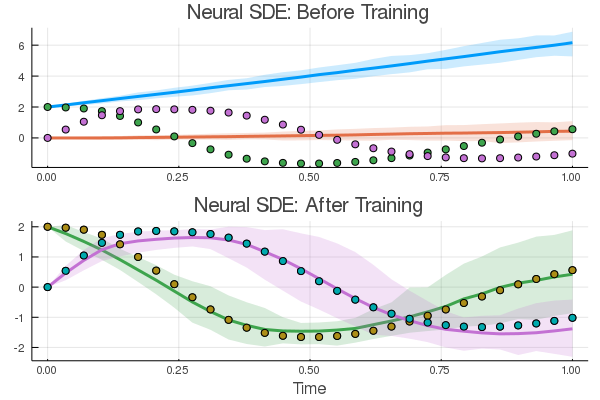
And there we go: a neural dynamical system that fits both the mean and variance of the timeseries data. Of course, there are a million other loss functions to explore, with millions of different properties. And universal stochastic differential equation structures. But we'll leave this for the reader!
Linking SDEs to PDEs: Kolmogorov Forward Equation Derivation
The Kolmogorov Forward Equation, also known to Physicists as the Fokker-Planck Equation, is important because it describes the time evolution of the probability density function. Whereas the stochastic differential equation describes how one trajectory of the stochastic processes evolves, the Kolmogorov Forward Equation describes how, if you were to be running many different simulations of the trajectory, the percent of trajectories that are around a given value evolves with time.
We will derive this for the arbitrary drift process:
\[ dx=f(x)dt+\sum_{i=1}^{m}g_{i}(x)dW_{i}. \]
Let $\psi(x)$ be an arbitrary time-independent transformation of $x$. Applying Ito's lemma for an arbitrary function we get
\[ d\psi(x,t)=\left(f(x,t)\frac{\partial\psi}{\partial x}+\frac{1}{2}\sum_{i=1}^{n}g_{i}^{2}(x,t)\frac{\partial^{2}\psi}{\partial x^{2}}\right)dt+\frac{\partial\psi}{\partial x}\sum_{i=1}^{n}g_{i}(x,t)dW_{i} \]
Take the expectation of both sides. Because expectation is a linear operator, we can move it inside the derivative operator to get:
\[ \frac{d}{dt}\mathbb{E}\left[\psi(x)\right]=\mathbb{E}\left[\frac{\partial\psi}{\partial x}f(x)\right]+\frac{1}{2}\mathbb{E}\left[\sum_{i=1}^{m}\frac{\partial^{2}\psi}{\partial x^{2}}g_{i}^{2}(x)\right]. \]
Notice that $\mathbb{E}\left[dW_{i}\right]=0$ and thus the differential Wiener terms dropped out.
Recall the definition of expected value is
\[ \mathbb{E}\left[\psi(x)\right]=\int_{-\infty}^{\infty}\rho(x,t)\psi(x)dx \]
where $\rho(x,t)$ is the probability density of equaling $x$ at a time $t$. Thus we get that the first term as:
\[ \frac{d}{dt}\mathbb{E}\left[\psi(x)\right]=\int_{-\infty}^{\infty}\frac{\partial\rho}{\partial t}\psi(x)dx \]
For the others, notice
\[ \mathbb{E}\left[\frac{\partial\psi}{\partial x}f(x)\right]=\int_{-\infty}^{\infty}\rho(x,t)\frac{\partial\psi}{\partial x}f(x)dx. \]
We rearrange terms doing integration by parts. Let $u=\rho f$ and $dv=\frac{\partial\psi}{\partial x}$. Thus $du=\frac{\partial(\rho f)}{\partial x}$ and $v=\psi$. Therefore we get that:
\[ \mathbb{E}\left[\frac{\partial\psi}{\partial x}f(x)\right]=\left[\rho f\psi\right]_{-\infty}^{\infty}-\int_{-\infty}^{\infty}\frac{\partial(\rho f)}{\partial x}\psi(x)dx. \]
In order for the probability distribution to be bounded (which it must be: it must integrate to 1), $\rho$ must vanish at both infinities. Thus, assuming bounded expectation, $\mathbb{E}\left[\frac{\partial\psi}{\partial x}f(x)\right]<\infty$, we get that
\[ \mathbb{E}\left[\frac{\partial\psi}{\partial x}f(x)\right]=-\int_{-\infty}^{\infty}\frac{\partial(\rho f)}{\partial x}\psi(x)dx. \]
The next term we manipulate similarly,
\[ \begin{eqnarray*} \mathbb{E}\left[\frac{\partial\psi^{2}}{\partial x^{2}}g_{i}^{2}(x)\right] & = & \int_{-\infty}^{\infty}\frac{\partial^{2}\psi}{\partial x^{2}}g_{i}^{2}(x)\rho(x,t)dx\\ & = & \left[\rho g^{2}\frac{\partial\psi}{\partial x}\right]_{-\infty}^{\infty}-\int_{-\infty}^{\infty}\frac{\partial\left(g_{i}^{2}(x)\rho(x,t)\right)}{\partial x}\frac{\partial\psi}{\partial x}dx\\ & = & \left[\rho g^{2}\frac{\partial\psi}{\partial x}\right]_{-\infty}^{\infty}-\left[\frac{\partial\left(\rho g^{2}\right)}{\partial x}\psi\right]_{-\infty}^{\infty}+\frac{1}{2}\int_{-\infty}^{\infty}\frac{\partial^{2}\left(g_{i}^{2}(x)\rho(x,t)\right)}{\partial x^{2}}\psi(x)dx\\ & =\frac{1}{2} & \int_{-\infty}^{\infty}\frac{\partial^{2}\left(g_{i}^{2}(x)\rho(x,t)\right)}{\partial x^{2}}\psi(x)dx \end{eqnarray*} \]
where we note that, at the edges, the derivative of $\rho$ converges to zero since $\rho$ converges to 0 and thus the constant terms vanish. Thus we get that
\[ \int_{-\infty}^{\infty}\frac{\partial\rho}{\partial t}\psi(x)dx=-\int_{-\infty}^{\infty}\frac{\partial(\rho f)}{\partial x}\psi(x)dx+\frac{1}{2}\sum_{i}\int_{-\infty}^{\infty}\frac{\partial(g_{i}^{2}\rho)}{\partial x}\psi(x)dx \]
which we can re-write as
\[ \int_{-\infty}^{\infty}\left(\frac{\partial\rho}{\partial t}+\frac{\partial(\rho f)}{\partial x}-\frac{1}{2}\sum_{i}\frac{\partial(g_{i}^{2}\rho)}{\partial x}\right)\psi(x)dx=0. \]
Since $\psi(x)$ is arbitrary, let $\psi(x)=I_{A}(x)$, the indicator function for the set $A$:
\[ I_{A}(x)=\begin{cases} 1, & x\in A\\ 0 & o.w. \end{cases} \]
Thus we get that:
\[ \int_{A}\left(\frac{\partial\rho}{\partial t}+\frac{\partial(\rho f)}{\partial x}-\frac{1}{2}\sum_{i}\frac{\partial(g_{i}^{2}\rho)}{\partial x}\right)dx=0 \]
for any arbitrary $A\subseteq\mathbb{R}$. Notice that this implies that the integrand must be identically zero. Thus
\[ \frac{\partial\rho}{\partial t}+\frac{\partial(\rho f)}{\partial x}-\frac{1}{2}\sum_{i}\frac{\partial(g_{i}^{2}\rho)}{\partial x}=0, \]
which we re-arrange as
\[ \frac{\partial\rho(x,t)}{\partial t}=-\frac{\partial}{\partial x}[f(x)\rho(x,t)]+\frac{1}{2}\sum_{i=1}^{m}\frac{\partial^{2}}{\partial x^{2}}\left[g_{i}^{2}(x)\rho(x,t)\right], \]
which is the Forward Kolmogorov or the Fokker-Planck equation.
Example Application: Ornstein–Uhlenbeck Process
Consider the stochastic process:
\[ dx=-xdt+dW_{t}, \]
where $W_{t}$ is Brownian motion. The Forward Kolmogorov Equation for this SDE is thus:
\[ \frac{\partial\rho}{\partial t}=\frac{\partial}{\partial x}(x\rho)+\frac{1}{2}\frac{\partial^{2}}{\partial x^{2}}\rho(x,t) \]
Assume that the initial conditions follow the distribution $u$ to give:
\[ \rho(x,0)=u(x) \]
and the boundary conditions are absorbing at infinity. To solve this PDE, let $y=xe^{t}$ and apply Ito's lemma
\[ dy=xe^{t}dt+e^{t}dx=e^{t}dW \]
and notice this follows has the Forward Kolmogorov Equation
\[ \frac{\partial\rho}{\partial t}=\frac{e^{2t}}{2}\frac{\partial^{2}\rho}{\partial y^{2}}. \]
which is a simple form of the Heat Equation. If $\rho(x,0)=\delta(x)$, the Dirac-$\delta$ function, then we know this solves as a Gaussian with diffusion constant $\frac{e^{2t}}{2}$ to give us:
\[ \rho(y,t)=\frac{1}{\sqrt{2\pi e^{2t}t}}e^{-\frac{y^{2}}{2e^{2t}t}}. \]
and thus $y\sim N(0,e^{2t}t)$.
The Two Way Meaning: Feynman-Kac Theorem
The derivation of the Kolmogorov equations is a two-way street. One way to solve a specific set of parabolic PDEs, the quasilinear diffusion-advection equations, is to solve a bunch of SDEs and look at the probability distributions. If 100 spatial points in each dimension were required for the correct accuracy, then it would take $(64 \times 100)^100$ bits, or
https://www.wolframalpha.com/input/?i=%2864*100%29%5E100+bits+as+terabytes
\[ 5 \times 10^{367} \]
terabytes of memory! However, just a system of 100 SDEs can be solved very easily. Exploiting this direction is known as the Feynman-Kac Theroem and it's commonly used in physical applications.
Meanwhile, Monte Carlo methods can have slow convergence, so if you only have 3 SDEs, then it can be much faster to solve the diffusion-advection equations to get the probability distributions. This two sided view of parabolic PDEs, as both a local SDE or a global PDE, can be exploited for computational gains.
Side Note
Hyperbolic PDEs have a different relation, known as the Method of Characteristics, which turns global PDEs into local ODEs.
Terminal PDEs and Forward-Backwards SDEs
The downside of Feynman-Kac is that it only applies to a very specific set of PDEs: the quasilinear diffusion advection equation that we derived. However, what if we wanted to solve high dimensional PDEs of an expanded form? It turns out there is some theory that links more partial differential equations to SDEs.
Consider the class of semilinear parabolic PDEs, in finite time $t\in[0, T]$ and $d$-dimensional space $x\in\mathbb R^d$, that have the form
\[ \begin{align} \frac{\partial u}{\partial t}(t,x) &+\frac{1}{2}\text{trace}\left(\sigma\sigma^{T}(t,x)\left(\text{Hess}_{x}u\right)(t,x)\right)\\ &+\nabla u(t,x)\cdot\mu(t,x) \\ &+f\left(t,x,u(t,x),\sigma^{T}(t,x)\nabla u(t,x)\right)=0,\end{align} \]
with a terminal condition $u(T,x)=g(x)$. In this equation, $\text{trace}$ is the trace of a matrix, $\sigma^T$ is the transpose of $\sigma$, $\nabla u$ is the gradient of $u$, and $\text{Hess}_x u$ is the Hessian of $u$ with respect to $x$. Furthermore, $\mu$ is a vector-valued function, $\sigma$ is a $d \times d$ matrix-valued function and $f$ is a nonlinear function. We assume that $\mu$, $\sigma$, and $f$ are known.
We wish to find the solution at initial time, $t=0$, at some starting point, $x = \zeta$.
Why the Terminal PDE?
A PDE where we only know the final value? This may sound contrived, but in reality this is a very natural PDE, because it turns out to be the general form of stochastic optimal control problems. So if you could solve it effectively, you could solve both determinsitic and stochastic optimal control in a very efficient way!
Terminal PDEs in Finance and Economics
It turns out that there is a large class of problems in economics and finance that satisfy this form. The reason is because in these problems you may know the value of something at the end, when you're going to sell it, and you want to evaluate it right now. The classic example is in options pricing. An option is a contract to be able to solve a stock at a given value. The simplest case is a contract that can only be executed at a pre-determined time in the future. Let's say we have an option to sell a stock at 100 no matter what. This means that, if the stock at the strike time (the time the option can be sold) is 70, we will make 30 from this option, and thus the option itself is worth 30. The question is, if I have this option today, the strike time is 3 months in the future, and the stock price is currently 70, how much should I value the option today?
To solve this, we need to put a model on how we think the stock price will evolve. One simple version is a linear stochastic differential equation, i.e. the stock price will evolve with a constant interest rate $r$ with some volitility (randomness) $\sigma$, in which case:
\[ dX_t = r X_t dt + \sigma X_t dW_t. \]
From this model, we can evaluate the probability that the stock is going to be at given values, which then gives us the probability that the option is worth a given value, which then gives us the expected (or average) value of the option. This is the Black-Scholes problem. However, a more direct way of calculating this result is writing down a partial differential equation for the evolution of the value of the option $V$ as a function of time $t$ and the current stock price $x$. At the final time point, if we know the stock price then we know the value of the option, and thus we have a terminal condition $V(T,x) = g(x)$ for some known value function $g(x)$. The question is, given this value at time $T$, what is the value of the option at time $t=0$ given that the stock currently has a value $x = \zeta$. Why is this interesting? This will tell you what you think the option is currently valued at, and thus if it's cheaper than that, you can gain money by buying the option right now! This means that the "solution" to the PDE is the value $V(0,\zeta)$, where we know the final points $V(T,x) = g(x)$.
Nonlinear Black-Scholes as a Semilinear Parabolic PDEs
Now let's look at a few applications which have PDEs that are solved by this method. One set of problems that are solved, given our setup, are Black-Scholes types of equations. Unless a lot of previous literature, this works for a wide class of nonlinear extensions to Black-Scholes with large portfolios. Here, the dimension of the PDE for $V(t,x)$ is the dimension of $x$, where the dimension is the number of stocks in the portfolio that we want to consider. If we want to track 1000 stocks, this means our PDE is 1000 dimensional! Traditional PDE solvers would need around $N^{1000}$ points evolving over time in order to arrive at the solution, which is completely impractical.
One example of a nonlinear Black-Scholes equation in this form is the Black-Scholes equation with default risk. Here we are adding to the standard model the idea that the companies that we are buying stocks for can default, and thus our valuation has to take into account this default probability as the option will thus become value-less. The PDE that is arrived at is:
\[ \frac{\partial u}{\partial t}(t,x) + \bar{\mu}\cdot \nabla u(t, x) + \frac{\bar{\sigma}^{2}}{2} \sum_{i=1}^{d} \left |x_{i} \right |^{2} \frac{\partial^2 u}{\partial {x_{i}}^2}(t,x) \\ - (1 -\delta )Q(u(t,x))u(t,x) - Ru(t,x) = 0 \]
with terminating condition $g(x) = \min_{i} x_i$ for $x = (x_{1}, . . . , x_{100}) \in R^{100}$, where $\delta \in [0, 1)$, $R$ is the interest rate of the risk-free asset, and Q is a piecewise linear function of the current value with three regions $(v^{h} < v ^{l}, \gamma^{h} > \gamma^{l})$,
\[ \begin{align} Q(y) &= \mathbb{1}_{(-\infty,\upsilon^{h})}(y)\gamma ^{h} + \mathbb{1}_{[\upsilon^{l},\infty)}(y)\gamma ^{l} \\ &+ \mathbb{1}_{[\upsilon^{h},\upsilon^{l}]}(y) \left[ \frac{(\gamma ^{h} - \gamma ^{l})}{(\upsilon ^{h}- \upsilon ^{l})} (y - \upsilon ^{h}) + \gamma ^{h} \right ]. \end{align} \]
This PDE can be cast into the general PDE form by setting:
\[ \begin{align} \mu &= \overline{\mu} X_{t} \\ \sigma &= \overline{\sigma} \text{diag}(X_{t}) \\ f &= -(1 -\delta )Q(u(t,x))u(t,x) - R u(t,x) \end{align} \]
Stochastic Optimal Control as a Deep BSDE Application
Another type of problem that fits into this terminal PDE form is the stochastic optimal control problem. The problem is a generalized context to what motivated us before. In this case, there are a set of agents which undergo some known stochastic model. What we want to do is apply some control (push them in some direction) at every single timepoint towards some goal. For example, we have the physics for the dynamics of drone flight, but there's randomness in the wind condition, and so we want to control the engine speeds to move in a certain direction. However, there is a cost associated with controling, and thus the question is how to best balance the use of controls with the natural stochastic evolution.
Formally, optimal control is defined finding a $u(t)$ such that for
\[ X' = f(X,u,t) \]
we minimize some objective. That is, $X$ satisfies some differential equation, $u$ can modify it, and we want to minimize some cost on the solution. In many cases this cost can include a penalty on "using" $u$. For example, a cost for the amount of energy used when doing advanced drone maneuvers. Stochastic optimal control is the case where:
\[ dX_t = f(X_t,u_t,t)dt + g(X_t,u_t,t)dW_t \]
that is, the underlying driving process is a stochastic differential equation.
We can represent the global solution to the optimal control as $u(t,x)$, i.e. what should we be doing to the system at time $t$ if $X=x$. It turns out this is in the same form as the Black-Scholes problem. There is a model evolving forwards, and when we get to the end we know how much everything "cost" because we know if the drone got to the right location and how much energy it took. So in the same sense as Black-Scholes, we can know the value at the end and try and propogate it backwards given the current state of the system $x$, to find out $u(0,\zeta)$, i.e. how should we control right now given the current system is in the state $x = \zeta$. It turns out that the solution of $u(t,x)$ where $u(T,x)=g(x)$ is given and we want to find $u(0,\zeta)$ is given by a partial differential equation which is known as the Hamilton-Jacobi-Bellman equation, which is one of these terminal PDEs that is representable by the parabolic PDE form above!
Take the classical linear-quadratic Gaussian (LQG) control problem in 100 dimensions
\[ dX_t = 2\sqrt{\lambda} c_t dt + \sqrt{2} dW_t \]
with $t\in [0,T]$, $X_0 = x$, and with a cost function
\[ C(c_t) = \mathbb{E}\left[\int_0^T \Vert c_t \Vert^2 dt + g(X_t) \right] \]
where $X_t$ is the state we wish to control, $\lambda$ is the strength of the control, and $c_t$ is the control process. To minimize the control, the Hamilton–Jacobi–Bellman equation:
\[ \frac{\partial u}{\partial t}(t,x) + \Delta u(t,x) - \lambda \Vert \nabla u(t,x) \Vert^2 = 0 \]
has a solution $u(t,x)$ which at $t=0$ represents the optimal cost of starting from $x$.
This PDE can be rewritten into the canonical form of \Cref{pdeform} by setting:
\[ \begin{align} \mu &= 0, \\ \sigma &= \overline{\sigma} I, \\ f &= -\alpha \left \| \sigma^T(s,X_s)\nabla u(s,X_s)) \right \|^{2}, \end{align} \]
where $\overline{\sigma} = \sqrt{2}$, T = 1 and $X_0 = (0,. . . , 0) \in R^{100}$.
Solving Semilinear Parabolic PDEs with Universal Stochastic Differential Equations
Consider the class of semilinear parabolic PDEs, in finite time $t\in[0, T]$ and $d$-dimensional space $x\in\mathbb R^d$, that have the form
\[ \begin{align} \frac{\partial u}{\partial t}(t,x) &+\frac{1}{2}\text{trace}\left(\sigma\sigma^{T}(t,x)\left(\text{Hess}_{x}u\right)(t,x)\right)\\ &+\nabla u(t,x)\cdot\mu(t,x) \\ &+f\left(t,x,u(t,x),\sigma^{T}(t,x)\nabla u(t,x)\right)=0,\end{align} \]
with a terminal condition $u(T,x)=g(x)$. Let $W_{t}$ be a Brownian motion and take $X_t$ to be the solution to the stochastic differential equation
\[ dX_t = \mu(t,X_t) dt + \sigma (t,X_t) dW_t \]
with initial condition $X(0)=\zeta$. We know from our derivation above that, if everything was linear (and $f=0$), then the PDE is locally represented by the SDE of $X(t)$. However, some smart people have recognized that, while this form cannot be represented as the SDE $X(t)$, it can be represented by augmenting the SDE $X(t)$ with an extra term defined in reverse, known as the backwards SDE or BSDE:
\[ \begin{align} u(t, &X_t) - u(0,\zeta) = \\ & -\int_0^t f(s,X_s,u(s,X_s),\sigma^T(s,X_s)\nabla u(s,X_s)) ds \\ & + \int_0^t \left[\nabla u(s,X_s) \right]^T \sigma (s,X_s) dW_s,\end{align} \]
with terminating condition $g(X_T) = u(X_T,W_T)$. Note that this $W_s$ is the same Brownian motion as the forward process. Indeed it makes sense given the example problems since the control $u(t)$ should be dependent on "the current randomness"
Notice that we can put these terms together with the forward SDE to get what's known as the forward-backward SDE (FBSDE):
\[ \begin{aligned} dX_t =& \mu(t,X_t) dt + \sigma (t,X_t) dW_t,\\ dU_t =& f(t,X_t,U_t,\sigma^T (t,X_t) \nabla u(t,X_t)) dt\\ &+ \left[\sigma^T (t,X_t) \nabla u(t,X_t)\right]^T dW_t,\end{aligned} \]
However, we don't know what $\sigma^T (t,X_t) \nabla u(t,X_t)$ is without solving or repsenting the PDE! Also, since the $u(t)$ term is ran in reverse, we know its final condition (if we know the final X(t) value!), but we don't know its initial condition! So to handle this, let's represent everything that we don't know with neural networks, i.e.
\[ \begin{align} dX_t &= \mu(t,X_t) dt + \sigma (t,X_t) dW_t,\\ dU_t &= f(t,X_t,U_t,U^1_{\theta_1}(t,X_t)) dt + \left[U^1_{\theta_1}(t,X_t)\right]^T dW_t,\end{align} \]
where $U^1$ is some universal approximator and $u(0,X_0) = U^2(X_0)$ is some other universal approximator.
How do we train these universal approximators? Well, we need to make sure the terminating condition holds, i.e. $g(X_T) = u(X_T,W_T)$, and thus we make our cost be the difference of these values:
\[ C(\theta) = E\left[g(X_t) - u(X_T,W_T)\right] \]
which means we solve the FBSDE a few times and check on average how the terminating condition is doing. If our parameters start to cause the terminating condition to "essentially" hold, then $U^1 \approx \sigma^T (t,X_t) \nabla u(t,X_t)$ and $U^2 \approx u(0,X_0)$, and thus we know the solution to the FBSDE.
But what about the PDE? The goal was to find the solution at initial time, $t=0$ with some starting point, $X_0 = \zeta$. Therefore the solution to the terminal PDE, after training the neural networks, is simply $U^2(X_0)$!
Universal SDE Solving Semilinear Parabolic PDEs
Example codes for doing this can be found in NeuralNetDiffEq.jl.